Building Simple AIS Aggregations

Rory Meyer Jan 26, 2021

When trying to derive meaningful information from AIS data some users are often interested in long term trends rather than data from a specific message from a specific vessels. Aggregations allow millions/billions/unwieldy amounts of small data chunks to be processed into more usable collections. When talking about geo-spatial aggregations this is generally done by collecting data that falls into spatial areas, whether user defined grids, legal boundaries or ecological definitions.

In this example I’ll be taking AIS data for vessels travelling through the Southern Atlantic Ocean, creating a pleasant hexagon grid (thanks PostGIS 3.1) and then collecting data over this for a specific date.

From an the PostGIS documentation on Hex Grids

How the data is collected is up to the developer/scientist/user. It can be as simple as just counting the number of AIS messages that fall into each hexagon or as complex as building a trajectory of each vessel, laying it over the grid and allocating weighting to each cell as determined by the portion of the trajectory covering the cell (more on this later). Simple aggregations are often quick, easy and provide some information that looks good but *could* hide or distort the data.

If you just added up the AIS messages received in each grid cell what would be measured? Most users are interested in vessel density in order to measure things like pollution, fishing effort, port activity etc but straight up counts of AIS messages often results in a measure of reception strength… You see, the messages that are recorded in the database are not a complete set of messages that have been transmitted. Land based receivers often receive messages from vessels every couple of minutes (depending on activity, transmitter class, rate of turn etc etc) while satellite receivers receive messages when they’re overhead. It’s often a good idea to get away from the individual messages and treat the data as irregularly sampled points along a trajectory.

Okay, but back to the hex grid. I’ve built up a DB with some ocean defined geometry from the Marine Regions website. These are pulled into a PostgreSQL + PostGIS 3.1 +TimeScaleDB 2.0 database (don’t worry about TimeScaleDB for now, it’s got some nifty functions that deal with insertion, storage and querying of time-series data).

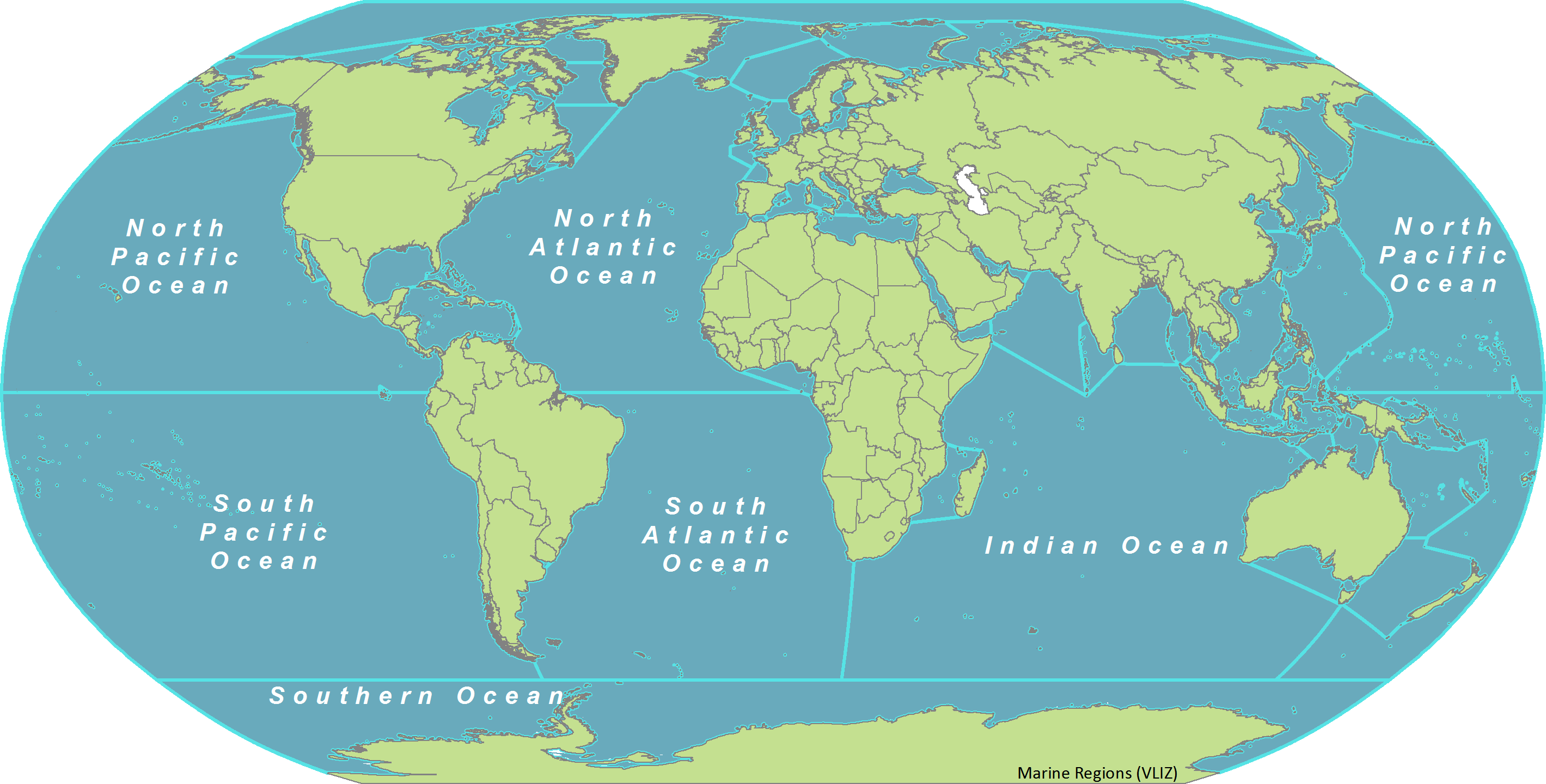
IHO Sea Areas from Flanders Marine Institute

So some basic code to generate the hex grid could be:

SELECT  
	hex.geom
FROM
        geo.ocean_geom
CROSS JOIN 
        ST_HexagonGrid(10, ocean_geom.geom) AS hex
WHERE   ST_Intersects(ocean_geom.geom, hex.geom)
AND     geoname = 'South Atlantic Ocean';

but this causes an error:

ERROR:  GEOSIntersects: TopologyException: side location conflict at -62.263198463199373 -39.87260466882973

Looking at the location reported the error, and eyeballing this in QGIS doesn’t show anything too significant. It’s a piece of knotty coast off of South America. It might just be as simple as 2 vertices occupying the same place and luckily QGIS has a method of checking what’s up:

SELECT 
	st_isvalid(ocean_geom.geom),
	ST_IsValidReason(ocean_geom.geom)
FROM    geo.ocean_geom
WHERE   geoname = 'South Atlantic Ocean'

shows “Self-intersection[-62.2631984631994 -39.8726046688297]”.

Ah, okay. PostGIS can handle that. And why not simplify the geometry while we’re at it so that generation of the grid will go a little quicker:

With geom_of_interest as 
(SELECT 
	ST_MakeValid(ST_Simplify(geom,1)) as valid_geom
FROM geo.ocean_geom 
WHERE geoname = 'South Atlantic Ocean')

SELECT 
	ST_AsText(hex.geom), 
	hex.geom
FROM
    geom_of_interest
CROSS JOIN
    ST_HexagonGrid(1, ST_Envelope(valid_geom)) AS hex
WHERE
    ST_Within(hex.geom, valid_geom)

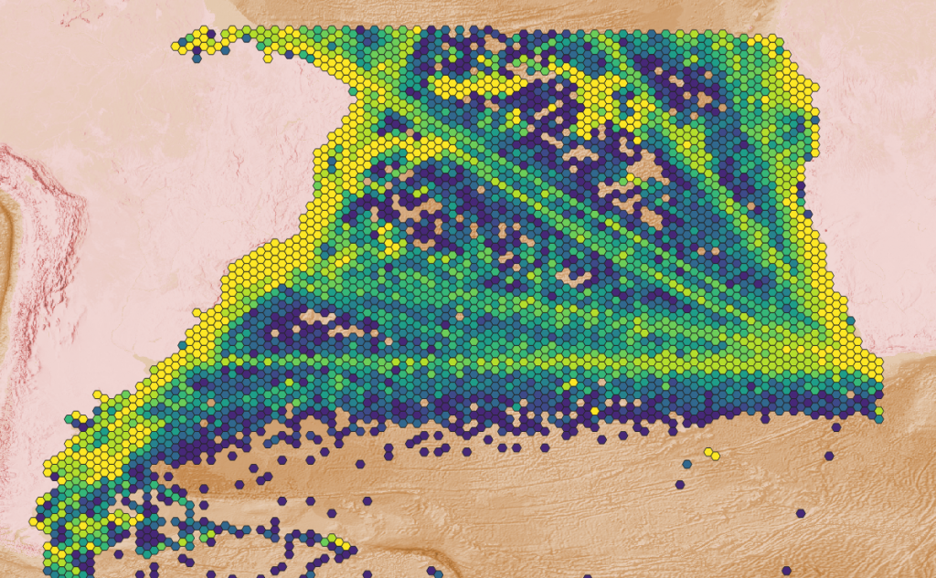
Keep in mind we’re operating in SRID:4326 here, so all the simplify and size arguments are in degrees. 1 degree ~ 110 km’s. This generation took around 9 seconds, not great but not the end of the world and created a hex grid like this:

Some distortions near the Antarctic due to the projection and some around the coast and islands due to the St_Within filter.

Using a combo ST_Within OR ST_Overlaps filter fixes that, while only adding another 2 seconds to the query:

Now for it all together, with some materialization and indexes to speed things up:

DROP MATERIALIZED VIEW IF EXISTS geo.hex_grid;
CREATE MATERIALIZED VIEW geo.hex_grid AS
With geom_of_interest as 
(SELECT 
	ST_MakeValid(ST_Simplify(geom,1)) as valid_geom
FROM geo.ocean_geom 
WHERE geoname = 'South Atlantic Ocean')
 
SELECT  
	  ST_AsText(hex.geom), 
	  hex.geom
FROM
      geom_of_interest 
CROSS JOIN
      ST_HexagonGrid(0.5, ST_Envelope(valid_geom)) AS hex
WHERE ST_Within(hex.geom, valid_geom)
OR    ST_Overlaps(hex.geom, valid_geom);

CREATE INDEX ON geo.hex_grid USING gist (geom);

	
SELECT 
	St_AsText(hex_grid.geom) AS wkt,
	hex_grid.geom,
	count(*)
FROM ais.daily_pos_cagg
JOIN geo.hex_grid
ON ST_Within(daily_pos_cagg.position, hex_grid.geom)
WHERE daily_pos_cagg.day BETWEEN '2020-01-01' AND '2020-02-01'
GROUP BY hex_grid.geom

Now this isn’t a very useful aggregation. But it’s a start.

Citations

Flanders Marine Institute (2018). IHO Sea Areas, version 3. Available online at https://www.marineregions.org/. https://doi.org/10.14284/323.